Simple analyses
Node activities
In this section we show how we can use the proposed operations with temporal quantities (the addition) for a simple analysis of temporal networks.
Assume that the values in temporal quantities auv from a temporal network matrix A are positive real numbers measuring the intensity of the activity of the node u on the node v. We define the activity of a group of nodes V1 on a group V2 (using the combinatorial semiring) as
act(V1,V2) = ∑{u∈V1 : ∑{v∈V2 : auv } } .
To illustrate the notion of activity we applied it on Franzosi's violence temporal network \citep{RF}. Roberto Franzosi collected from the journal news in the period (January 1919 - December 1922) information about the different types of interactions between political parties and other groups of people in Italy. The violence network contains only the data about violent actions and counts the number of interactions per month.
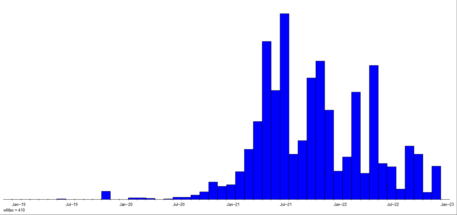
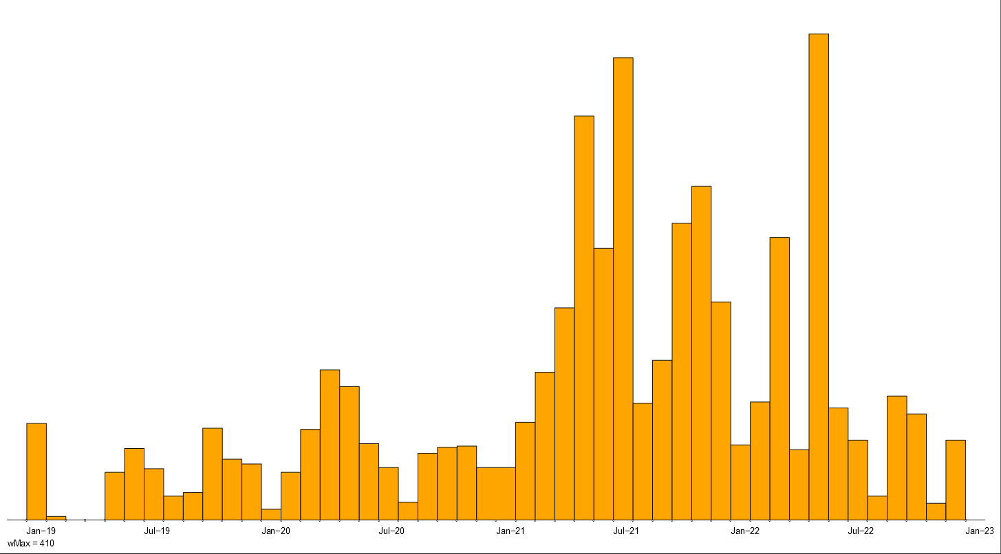
Intensity of violent activities of police, fascists and all.
We determined the temporal quantities
pol = act({police}, V) + act(V, {police}),
fas = act({fascists}, V) + act(V, {fascists}), and
all = act(V, V) .
They are presented in Figure~\ref{viol}. Comparing the intensity charts of police and fascists activity with overall activity we see that most of the violent activities in the first two years 1919 and 1920 were related to the police. In the next two years (1921 and 1922) they were taken over by the fascists.
>>> V = TQ.Ianus2Mat('./violence/violence.ten')
>>> list(V.keys())
['met', 'tit', 'til', 'typ', 'tin', 'mat', 'dim', 'nam']
>>> A = V['mat']
>>> TQ.MatSummary(A)
(1, 49, 1, 174)
>>> n = len(A); All = range(n)
>>> names = V['nam']; Times = V['til']
>>> for i,name in enumerate(names): print(i,name)
0 undefined
1 ?
2 people
3 police
4 land owners
5 anarchists
6 fascists
7 communists
8 workers (agricultural)
9 socialists
...
26 prisoners/arrested
27 foreigners
28 liberals
>>> # All-All
>>> ca = TQ.ActInt(A,All,All)
>>> # police - 3
>>> cb = TQ.sum(TQ.ActInt(A,[3],All),TQ.ActInt(A,All,[3]))
>>> # fascists - 6
>>> cc = TQ.sum(TQ.ActInt(A,[6],All),TQ.ActInt(A,All,[6]))
>>> comp = {}
>>> comp['All-All'] = ca
>>> comp['Pol-All'] = cb
>>> comp['Fas-All'] = cc
>>> comp['info']    = TQ.MatSummary(A)
>>> comp['lTimes']  = [lab for i,lab in Times]
>>> with open('violComp.json',mode='w',encoding='utf-8') as f:
   json.dump(comp,f,indent=2)
>>>
and drawing in R
> V <- fromJSON(file="violComp.json")
> names(V)
[1] "info"    "Fas-All" "All-All" "lTimes"  "Pol-All"
> V$info
[1]   1  49   1 174
> tMin <- V$info[1]; tMax <- V$info[2]; wMax <- 700
> lTimes <- V$lTimes
> times <- c(1,7,13,19,25,31,37,43,49)
> all <- V[[3]]; fas <- V[[2]]; pol <- V[[5]]
> plotTime(all,tMin,tMax,times,lTimes,wMax,h=250,main='All-All',col='orange')
> plotTime(pol,tMin,tMax,times,lTimes,wMax,h=250,main='Police',col='yellow')
> plotTime(fas,tMin,tMax,times,lTimes,wMax,h=250,main='Fascists',col='blue')
Products of a temporal matrix and a temporal vector
In some applications the product of a temporal matrix with a temporal vector is useful. There are two products - left and right.
Let A be a temporal matrix of size n✕m, v a vector of size n, and u a vector of size m. The product from left of A with v, denoted by u = v ● A, is defined by
uj = ⊕{i∈1:n : vi ⊙ aij }, j∈1:m
and the product from right of A with u, denoted by v = A ● u, is defined by
v_i = ⊕{j∈1:m : aij ⊙ uj}, i∈1:n .
In the TQ library both products are implemented as functions MatVecMulL(A,v) and
MatVecMulR(A,v).
If a vector v of size n is considered as a column vector - an n✕1 matrix - it holds
v ● A = (vT ⊙ A)T , and
A ● u = A ⊙ u .
T denotes the matrix transposition operation.
Temporal degrees
For an ordinary graph with a (binary) adjacency matrix A we can compute the corresponding indegree, i, and outdegree, o, vectors using (over the combinatorial semiring) the relations
i = e ● A and o = A ● e
where e is a column vector of size n = |V| with all its entries equal to 1. The same holds for temporal networks. In this case the vector e contains as values the temporal unit 1 = [(0,∞,1)].
This is the basis of TQ functions inDeg(A) and outDeg(A).
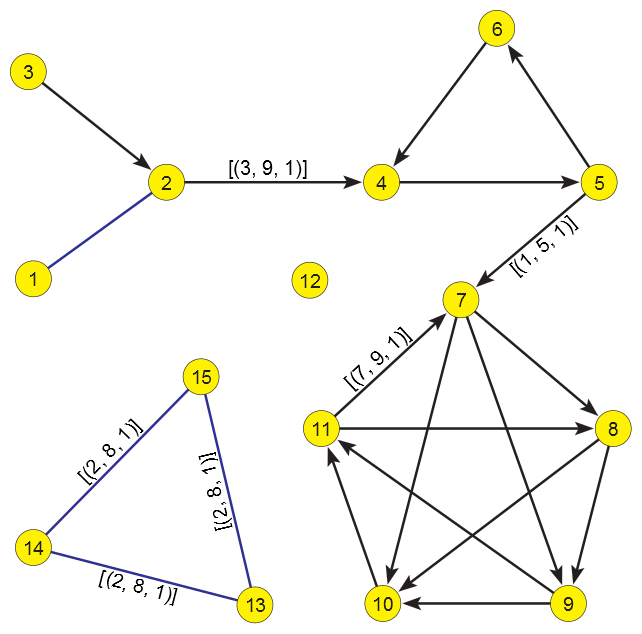
First example network testConn.net . All unlabeled links have a value of [(1,9,1)].
For a temporal network presented in Figure~\ref{graph} the corresponding temporal indegrees and outdegrees are given in following table:
Temporal indegrees and outdegrees for the first example network.
Indegrees	                      Outdegrees
 1 : [(1, 9, 1)]                  1 : [(1, 9, 1)]
 2 : [(1, 9, 2)]                  2 : [(1, 3, 1), (3, 9, 2)]
 3 : []                           3 : [(1, 9, 1)]
 4 : [(1, 3, 1), (3, 9, 2)]       4 : [(1, 9, 1)]
 5 : [(1, 9, 1)]                  5 : [(1, 5, 2), (5, 9, 1)]
 6 : [(1, 9, 1)]                  6 : [(1, 9, 1)]
 7 : [(1, 5, 1), (7, 9, 1)]       7 : [(1, 9, 3)]
 8 : [(1, 9, 2)]                  8 : [(1, 9, 2)]
 9 : [(1, 9, 2)]                  9 : [(1, 9, 2)]
10 : [(1, 9, 3)]                 10 : [(1, 9, 1)]
11 : [(1, 9, 2)]                 11 : [(1, 7, 1), (7, 9, 2)]
12 : []                          12 : []
13 : [(2, 8, 2)]                 13 : [(2, 8, 2)]
14 : [(2, 8, 2)]                 14 : [(2, 8, 2)]
15 : [(2, 8, 2)]                 15 : [(2, 8, 2)]
For example, the node 5 has in the time interval [1,5) outdegree 2. Because the arc (5,7) disappears at the time point 5 the outdegree of the node 5 diminishes to 1 in the interval [5,9).
>>> N = TQ.Ianus2Mat('./ten/testConn.ten')
>>> list(N.keys())
['met', 'tit', 'til', 'typ', 'tin', 'mat', 'dim', 'nam']
>>> A = N['mat']
>>> TQ.MatSummary(A)
(1, 9, 1, 1)
>>> id = TQ.inDeg(A); od = TQ.outDeg(A)
>>> TQ.VecList(id)
1 : [(1, 9, 1)]
2 : [(1, 9, 2)]
3 : []
4 : [(1, 3, 1), (3, 9, 2)]
5 : [(1, 9, 1)]
6 : [(1, 9, 1)]
7 : [(1, 5, 1), (7, 9, 1)]
8 : [(1, 9, 2)]
9 : [(1, 9, 2)]
10 : [(1, 9, 3)]
11 : [(1, 9, 2)]
12 : []
13 : [(2, 8, 2)]
14 : [(2, 8, 2)]
15 : [(2, 8, 2)]
>>> TQ.VecList(od)
1 : [(1, 9, 1)]
2 : [(1, 3, 1), (3, 9, 2)]
3 : [(1, 9, 1)]
4 : [(1, 9, 1)]
5 : [(1, 5, 2), (5, 9, 1)]
6 : [(1, 9, 1)]
7 : [(1, 9, 3)]
8 : [(1, 9, 2)]
9 : [(1, 9, 2)]
10 : [(1, 9, 1)]
11 : [(1, 7, 1), (7, 9, 2)]
12 : []
13 : [(2, 8, 2)]
14 : [(2, 8, 2)]
15 : [(2, 8, 2)]
>>>
We will use the simple temporal network from this section also for the illustration of some other algorithms because it allows the users to manually check the presented results.
Clustering coefficients
Let us assume that the network N is based on a simple directed graph G = (V, A) without loops. From a simple undirected graph we obtain the corresponding simple directed graph by replacing each edge with a pair of opposite arcs. In such a graph the clustering coefficient, C(v), of the node v is defined as the proportion between the number of realized arcs among the node's neighbors and the number of all possible arcs among the node's neighbors N(v), that is
C(v) = |A(N(v))| / ( k∙(k-1) )
where k is the number of neighbors of the node v. For a node v without neighbors or with a single neighbor we set C(v)=0.
The clustering coefficient measures a local density of the node's neighborhood. A problem with its applications in network analysis is that the identified densest neighborhoods are mostly very small. For this reason we provided in Pajek the corrected clustering coefficient, C'(v),
C'(v) = |A(N(v))| /( Δ∙(k-1) )
where Δ is the maximum number of neighbors in the network.
To count the number of realized arcs among the node's neighbors we use the observation that each arc forms a triangle with links from its end-nodes to the node v; and that the number of triangles in a simple undirected graph can be obtained as the diagonal value in the third power of the graph matrix (over the combinatorial semiring).
For simple directed graphs the counting of triangles is slightly more complicated.
Let us denote T = AT and S = A+T. Then the number of triangles can
be read from the diagonal of SAS .
This gives us a simple way to count the triangles which is used in the TQ function clusCoef(A,type=1) where the parameter type determines the type of normalization:
type = 1 - standard clustering coefficient; type = 2 - corrected clustering coefficient / temporal Δ; type = 3 - corrected clustering coefficient / overall Δ. The time complexity of the function clusCoef is O(n3 ∙ L).
Some useful functions:
nRows(A) returns the size (number of rows) of matrix A.
VecConst(n,v) constructs a vector of size n filled with the value v.
MatBin(A) transforms all values in the triples in the matrix A to 1.
MatSetDiag(A,c) sets all the diagonal entries of the matrix A to the value c.
MatSym(A) makes the transformation S = A⊕T.
VecSum(a,b) = [ai ⊕ bi, i∈1:n]
VecProd(a,b) = [ai ⊙ bi, i∈1:n]
VecInv(a) = [invert(ai), i∈1:n] in the combinatorial semiring.
invert(a) = [ (s,f,1/v) for (s,f,v) ∈ a ]
MatProd(A,B) determines the product A ⊙ B.
MatProdDiag(A,B) determines only the diagonal vector of the product A ⊙ B.
In the following tables the ordinary and the corrected clustering coefficients are presented for the first example network and its undirected skeleton.
Clustering coefficients for the first example network.
Clustering coefficient                  Corrected clustering coefficient
 1 : []                                  1 : []
 2 : []                                  2 : []
 3 : []                                  3 : []
 4 : [(1, 3, 0.5), (3, 9, 0.1667)]       4 : [(1, 3, 0.25), (3, 9, 0.125)]
 5 : [(1, 5, 0.1667), (5, 9, 0.5)]       5 : [(1, 5, 0.125), (5, 9, 0.25)]
 6 : [(1, 9, 0.5)]                       6 : [(1, 9, 0.25)]
 7 : [(1, 5, 0.25), (5, 9, 0.5)]         7 : [(1, 5, 0.25), (5, 7, 0.375),
                                              (7, 9, 0.5)]
 8 : [(1, 7, 0.4167), (7, 9, 0.5)]       8 : [(1, 7, 0.4167), (7, 9, 0.5)]
 9 : [(1, 7, 0.4167), (7, 9, 0.5)]       9 : [(1, 7, 0.4167), (7, 9, 0.5)]
10 : [(1, 7, 0.4167), (7, 9, 0.5)]      10 : [(1, 7, 0.4167), (7, 9, 0.5)]
11 : [(1, 9, 0.5)]                      11 : [(1, 7, 0.375), (7, 9, 0.5)]
12 : []                                 12 : []
13 : [(2, 8, 1.0)]                      13 : [(2, 8, 0.5)]
14 : [(2, 8, 1.0)]                      14 : [(2, 8, 0.5)]
15 : [(2, 8, 1.0)]                      15 : [(2, 8, 0.5)]
Clustering coefficients for the skeleton of the first example network.
Clustering coefficient                  Corrected clustering coefficient
 1 : []                                  1 : []
 2 : []                                  2 : []
 3 : []                                  3 : []
 4 : [(1, 3, 1.0), (3, 9, 0.3333)]       4 : [(1, 3, 0.5), (3, 9, 0.25)]
 5 : [(1, 5, 0.3333), (5, 9, 1.0)]       5 : [(1, 5, 0.25), (5, 9, 0.5)]
 6 : [(1, 9, 1.0)]                       6 : [(1, 9, 0.5)]
 7 : [(1, 5, 0.5), (5, 9, 1.0)]          7 : [(1, 5, 0.5), (5, 7, 0.75),
                                              (7, 9, 1.0)]
 8 : [(1, 7, 0.8333), (7, 9, 1.0)]       8 : [(1, 7, 0.8333), (7, 9, 1.0)]
 9 : [(1, 7, 0.8333), (7, 9, 1.0)]       9 : [(1, 7, 0.8333), (7, 9, 1.0)]
10 : [(1, 7, 0.8333), (7, 9, 1.0)]      10 : [(1, 7, 0.8333), (7, 9, 1.0)]
11 : [(1, 9, 1.0)]                      11 : [(1, 7, 0.75), (7, 9, 1.0)]
12 : []                                 12 : []
13 : [(2, 8, 1.0)]                      13 : [(2, 8, 0.5)]
14 : [(2, 8, 1.0)]                      14 : [(2, 8, 0.5)]
15 : [(2, 8, 1.0)]                      15 : [(2, 8, 0.5)]
And the corresponding Python code:
>>> N = TQ.Ianus2Mat('./ten/testConn.ten')
>>> list(N.keys())
['met', 'tit', 'til', 'typ', 'tin', 'mat', 'dim', 'nam']
>>> A = N['mat']
>>> cc1 = TQ.clusCoef(A)
>>> print("Clustering coefficient 1"); TQ.VecList(cc1)
Clustering coefficient 1
1 : []
2 : []
3 : []
4 : [(1, 3, 0.5), (3, 9, 0.16666666666666666)]
5 : [(1, 5, 0.16666666666666666), (5, 9, 0.5)]
6 : [(1, 9, 0.5)]
7 : [(1, 5, 0.25), (5, 9, 0.5)]
8 : [(1, 7, 0.41666666666666663), (7, 9, 0.5)]
9 : [(1, 7, 0.41666666666666663), (7, 9, 0.5)]
10 : [(1, 7, 0.41666666666666663), (7, 9, 0.5)]
11 : [(1, 9, 0.5)]
12 : []
13 : [(2, 8, 1.0)]
14 : [(2, 8, 1.0)]
15 : [(2, 8, 1.0)]
>>> cc2 = TQ.clusCoef(A,type=2)
>>> print("Clustering coefficient 2"); TQ.VecList(cc2)
Clustering coefficient 2
1 : []
2 : []
3 : []
4 : [(1, 3, 0.25), (3, 9, 0.125)]
5 : [(1, 5, 0.125), (5, 9, 0.25)]
6 : [(1, 9, 0.25)]
7 : [(1, 5, 0.25), (5, 7, 0.375), (7, 9, 0.5)]
8 : [(1, 7, 0.41666666666666663), (7, 9, 0.5)]
9 : [(1, 7, 0.41666666666666663), (7, 9, 0.5)]
10 : [(1, 7, 0.41666666666666663), (7, 9, 0.5)]
11 : [(1, 7, 0.375), (7, 9, 0.5)]
12 : []
13 : [(2, 8, 0.5)]
14 : [(2, 8, 0.5)]
15 : [(2, 8, 0.5)]
>>> S = TQ.MatSym(A)
>>> ccs1 = TQ.clusCoef(S)
>>> print("Clustering coefficient 1 / skeleton"); TQ.VecList(ccs1)
Clustering coefficient 1 / skeleton
1 : []
2 : []
3 : []
4 : [(1, 3, 1.0), (3, 9, 0.3333333333333333)]
5 : [(1, 5, 0.3333333333333333), (5, 9, 1.0)]
6 : [(1, 9, 1.0)]
7 : [(1, 5, 0.5), (5, 9, 1.0)]
8 : [(1, 7, 0.8333333333333333), (7, 9, 1.0)]
9 : [(1, 7, 0.8333333333333333), (7, 9, 1.0)]
10 : [(1, 7, 0.8333333333333333), (7, 9, 1.0)]
11 : [(1, 9, 1.0)]
12 : []
13 : [(2, 8, 1.0)]
14 : [(2, 8, 1.0)]
15 : [(2, 8, 1.0)]
>>> ccs2 = TQ.clusCoef(S,type=2)
>>> print("Clustering coefficient 2 / skeleton"); TQ.VecList(ccs2)
Clustering coefficient 2 / skeleton
1 : []
2 : []
3 : []
4 : [(1, 3, 0.5), (3, 9, 0.25)]
5 : [(1, 5, 0.25), (5, 9, 0.5)]
6 : [(1, 9, 0.5)]
7 : [(1, 5, 0.5), (5, 7, 0.75), (7, 9, 1.0)]
8 : [(1, 7, 0.8333333333333333), (7, 9, 1.0)]
9 : [(1, 7, 0.8333333333333333), (7, 9, 1.0)]
10 : [(1, 7, 0.8333333333333333), (7, 9, 1.0)]
11 : [(1, 7, 0.75), (7, 9, 1.0)]
12 : []
13 : [(2, 8, 0.5)]
14 : [(2, 8, 0.5)]
15 : [(2, 8, 0.5)]
>>>
TQ User guide <<< >>>


