Patterns
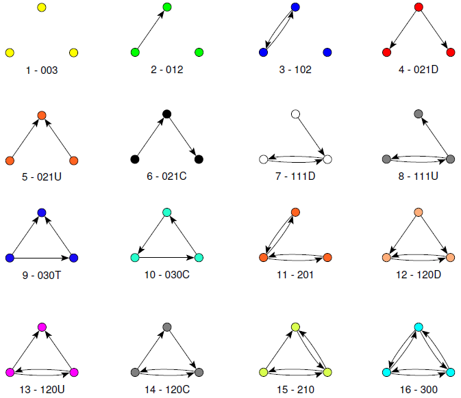
Dyadic census
library(statnet)
data(samplk)
gplot(samplk3,gmode="digraph")
dyad.census(samplk3) # M,A,N counts
dyad.census(network(samplk3,gmode="graph") # No As in undirected graphs
Triadic census
library(sna)
triad.census(samplk3) # Directed triad census
triad.census(samplk3,mode="graph") # Undirected triad census
Pattern search / Pajek
https://raw.githubusercontent.com/bavla/netstat/master/data/GED/frag16.paj
https://raw.githubusercontent.com/bavla/netstat/master/data/GED/Ragusan.ged
- Read GED file in Pajek
- Read Frag16.paj in Pajek
- Select GED network as Second
- Select first fragment as First
- Networks/Fragments (First in Second)
- Macro/Repeat last command [Fix Second Network] [15]
Counting with matrices
> library(statnet)
> data(florentine)
> A <- as.matrix(flomarriage)
> gplot(A,gmode="graph",displaylabels=TRUE)
> B <- A %*% A %*% A
> diag(B)
> (F2 <- sum(diag(B))/6)
> d <- degree(flomarriage)
> d1 <- d-1
> L <- as.edgelist.sna(flomarriage)
> head(L)
     [,1] [,2] [,3]
[1,]    1    9    1
[2,]    2    6    1
[3,]    2    7    1
[4,]    2    9    1
[5,]    3    5    1
[6,]    3    9    1
> (F3 <- as.numeric(d1[L[,1]] %*% d1[L[,2]] - 3*F2))
> (F4 <- sum(d*(d-1)*(d-2))/6)
> (F4 <- d %*% ((d-1)*(d-2))/6)
Orca
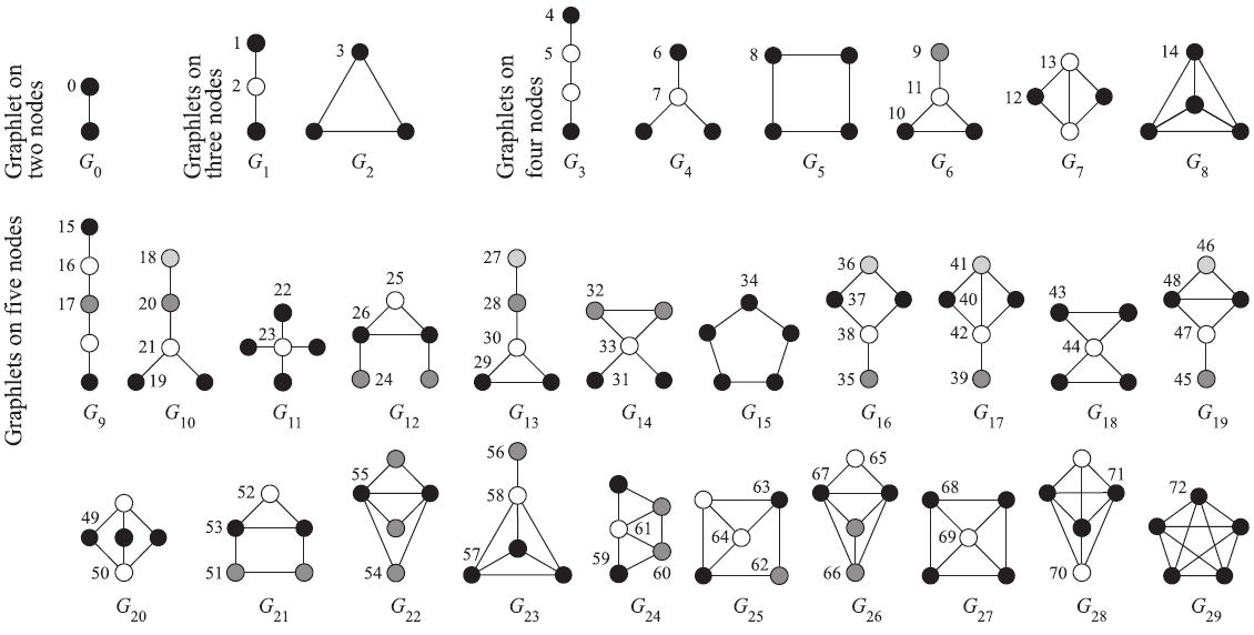
A graphlet census of a given graph can be computed using program orca. Download the orca.zip file and extract the compiled version for windows orca.exe into directory of your choice orcaDir. Details about the program orca are available in the paper.
Here is the partition of graphlets types to corresponding graphs Gi (both shifted for 1 - in R we start counting with 1):
p <- c(
 1, 2, 2, 3, 4, 4, 5, 5, 6, 7,  7, 7, 8, 8, 9,10,10,10,11,11,
11,11,12,12,13,13,13,14,14,14, 14,15,15,15,16,17,17,17,17,18,
18,18,18,19,19,20,20,20,20,21, 21,22,22,22,23,23,24,24,24,25,
25,25,26,26,26,27,27,27,28,28, 29,29,30 )
The input to program orca is a text file with numbers n (number of nodes)and m (number of edges) in the first line followed by
list of end-nodes of edges, each pair in its own line:
100 1000
41 67
34 0
69 24
78 58
62 64
5 45
...
Attention: nodes are numbered from 0 on.
Here we show how we can run the program orca from R:
> orcaDir <- "C:/Users/batagelj/Documents/papers/2018/moskva/NetR/progs/orca"
> orcaRun <- function(k=5,orcaData,orcaRes="orca.res"){
+   cmnd <- paste('"',orcaDir,'/orca.exe" ',k,' ',orcaData,' ',orcaRes,sep='')
+   system(cmnd,wait=TRUE)
+   G <- as.matrix(read.table(orcaRes))
+   colnames(G) <- paste("G",0:(ncol(G)-1),sep="")
+   rownames(G) <- paste("n",1:nrow(G),sep="")
+   return(G)
+ }
> setwd("C:/Users/batagelj/Documents/papers/2018/moskva/NetR/nets")
> k <- 4
> orcaData <- "../progs/orca/example.in"
> orcaRes <- "example.res"
> Gl <- orcaRun(k,orcaData,orcaRes)
nodes: 100
edges: 1000
max degree: 30
stage 1 - precomputing common nodes
0.00
stage 2 - counting full graphlets
0.00
stage 3 - building systems of equations
0.00
total: 0.00
> Gl[1:5,1:15]
   G0  G1  G2 G3   G4   G5   G6   G7  G8  G9  G10 G11 G12 G13 G14
n1 20 323 155 35 4054 3997 2031  609 500 512  912 437 114  89   5
n2 16 255  88 32 3574 2256 1604  212 270 410  849 257  90  82   9
n3 25 366 238 62 4362 5534 2144 1142 717 534 1480 908 168 232  18
n4 24 356 221 55 4337 5268 2109 1019 655 541 1308 816 151 173  16
n5 14 240  66 25 3232 1786 1651  139 236 405  700 156  81  63   6
To convert an sna network into orca file we can use the following function in R:
> library(sna)
> data(flo)
> gplot(flo,displaylabels=TRUE,usearrows=FALSE)
> gplot(flo,displaylabels=TRUE,gmode="graph")
> make.orcaInp <- function(G,orcaData){
+   out <- file(orcaData,"w")
+   N <- network(G,directed=FALSE)
+   cat(network.size(N),m <- network.edgecount(N),"\n",file=out)
+   L<-as.edgelist.sna(N)[,1:2]-1 # orca nodes start with 0
+   cat(paste(L[,1]," ",L[,2],"\n",sep="",collapse=""),file=out)
+   close(out)
+ }
> make.orcaInp(flo,"flo.in")
> GlFlo <- orcaRun(5,"flo.in","flo.res")
> row.names(GlFlo) <- row.names(flo)
> GlFlo[,1:15]
             G0 G1 G2 G3 G4 G5 G6 G7 G8 G9 G10 G11 G12 G13 G14
Acciaiuoli    1  5  0  0  6  0  9  0  0  1   0   0   0   0   0
Albizzi       3  8  3  0  6 14 12  1  1  1   0   0   0   0   0
Barbadori     2  7  1  0  8  7  9  0  0  2   0   0   0   0   0
Bischeri      3  6  2  1  8  9  4  0  0  0   1   1   1   0   0
Castellani    3  4  2  1  9  5  1  0  0  0   1   1   1   0   0
Ginori        1  2  0  0  8  0  1  0  0  0   0   0   0   0   0
Guadagni      4  6  6  0 11 16  1  4  1  2   0   0   0   0   0
Lamberteschi  1  3  0  0  6  0  3  0  0  0   0   0   0   0   0
Medici        6  6 14  1  9 26  1 16  1  0   2   4   0   0   0
Pazzi         1  1  0  0  5  0  0  0  0  0   0   0   0   0   0
Peruzzi       3  3  1  2  6  2  0  0  0  0   4   0   0   1   0
Pucci         0  0  0  0  0  0  0  0  0  0   0   0   0   0   0
Ridolfi       3  8  2  1  9 11  7  0  0  2   5   1   0   0   0
Salviati      2  5  1  0  5  5  9  0  0  1   0   0   0   0   0
Strozzi       4  4  4  2  9 10  0  1  0  1   2   2   0   1   0
Tornabuoni    3  8  2  1  9  9  9  0  1  0   5   1   0   0   0
PS. I just noticed that the Orca's authors prepared also an R package orca, paper. Take the above lines as an example how to link separate programs with R.
To do
- program in R a call to Pajek to search for selected fragments in a given network and import the results in R. example
- program in R graphlet distances

