Temporal quantities

Besides the presence/absence of nodes and links also their properties can change through time. To describe the changes we introduce the notion of a temporal quantity a with the activity set T_a ⊆ T

a'(t) = a(t) when t ∈ T_a, and a'(t) = ⌘ otherwise.

where a(t) is the value of a at an instant t, and ⌘ denotes the value undefined. In the following we will assume that a temporal quantity is extended in this way and we will use simply a to denote it.

We assume that the values of temporal quantities belong to a set A which is a semiring (A,⊕,⊙,0,1) for binary operations ⊕ : A✕A ⇢ A and ⊙ : A✕A ⇢ A \citep{GoMi,semi}. This means that (A,⊕,0) is an Abelian monoid - the addition ⊕ is associative and commutative, and has 0 as its neutral element; and (A,⊙,1) is a monoid - the multiplication ⊙ is associative and has 1 as its neutral element. Also, multiplication distributes from both sides over the addition.

Note that 0 and 1 denote the two elements of A that satisfy the required properties. In expressions the precedence of the multiplication ⊙ over the addition ⊕ is assumed. We can extend both operations to the set A_⌘ = A ⋃ { ⌘ } by requiring that for all a ∈ A_⌘ it holds

a ⊕ ⌘ = ⌘ ⊕ a = a and a ⊙ ⌘ = ⌘ ⊙ a = ⌘ .

The structure (A_⌘, ⊕, ⊙, ⌘, 1) is also a semiring.

The standard references on semirings are \cite{GaN} and \cite{GoMi}.

The “default” semiring is the combinatorial semiring (ℝ₀⁺, +, ∙, 0, 1) where + and ∙ are the usual addition and multiplication of real numbers.

In applications of semirings in the analysis of graphs and networks the addition ⊕ describes the composition of values on parallel walks and the multiplication ⊙ describes the composition of values on sequential walks

For the combinatorial semiring these two schemes correspond to basic principles of combinatorics: the Rule of Sum and the Rule of Product \citep{comb}.

In some applications other semirings are useful.

The semiring (ℝ^*, min, +, ∞, 0), where ℝ^* = ℝ₀⁺ ⋃ {∞}, is suitable to deal with the shortest paths problem in networks.

The semiring ({0, 1}, ⋁, ⋀, 0, 1) is used in solving reachability problems.

The semiring (ℝ, max, min, -∞, ∞)

In the following we shall use also the PathFinder semiring and geodetic semiring.

A default basic semiring is the combinatorial semiring. The current basic semiring operations ⊕ and ⊙ are in the TQ library available as functions sAdd(a,b) and sMul(a,b). The current basic semiring is changed by one of the functions combinatorial(), path(), maxmin(), reach(), PFsemi() and geodetic(). Data about the current semiring are displayed using the function report().

>>> TQ.report()
 
semiring =  combinatorial
add   =  add
mult  =  mul
sZero =  0
sOne  =  1
sN    =  []
sE    =  [(1, inf, 1)]
rPF   =  2 
 
>>> TQ.sAdd(3,4)
7
>>> TQ.sMul(3,4)
12
>>> TQ.PFsemi()
>>> TQ.sAdd(3,4)
3
>>> TQ.sMul(3,4)
5.0
>>> TQ.report()
 
semiring =  PFsemi
add   =  min
mult  =  pitagora
sZero =  inf
sOne  =  0
sN    =  []
sE    =  [(1, inf, 0)]
rPF   =  2 
 
>>> TQ.semiring
<function TQ.PFsemi at 0x00000000036F1730>
>>> TQ.sZero
inf
>>> TQ.inf+7
inf
>>> TQ.inf*TQ.inf
inf
>>>  

Let A_⌘(T) denote the set of all temporal quantities over A_⌘ in the time T. To extend the operations to networks and their matrices we first define the sum a ⊕ b (parallel links) as

(a ⊕ b)(t) = a(t) ⊕ b(t) and T_a⊕b = T_a ⋃ T_b;

and the product a ⊙ b (sequential links) as

(a ⊙ b)(t) = a(t) ⊙ b(t) and T_a⊙b = T_a ⋂ T_b.

In these definitions and also in the following text, to avoid the `pollution' with many different symbols, we use the symbols ⊕ and ⊙ to denote the semiring operations. The appropriate semiring can be determined from the context. For example, in the definition of addition of temporal quantities the symbol ⊕ on the left hand side of the equation operates on temporal quantities and the symbol ⊕ on the right hand side denotes the addition in the basic semiring A_⌘.

Let us define the temporal quantities 0 and 1 with requirements 0(t) = ⌘ and 1(t) = 1 for all t ∈ T. It is a routine task to verify that the structure (A_⌘(T), ⊕, ⊙, 0, 1) is also a semiring, and therefore so is the set of square matrices of order n over it for the addition A ⊕ B = S

s_ij = a_ij ⊕ b_ij

and multiplication A ⊙ B = P

p_ij = ⊕{k∈1:n : a_ik ⊙ b_kj} .

Again, the symbols ⊕ and ⊙ on the left hand side operate on matrices and on the right hand side in the semiring of temporal quantities.

The matrix multiplication is closely related to traveling on networks. Consider an entry p_ij in an instant t

p_ij(t) = ⊕{k∈1:n : a_ik(t) ⊙ b_kj(t)} .

For a value p_ij to be defined (different from ⌘) there should exist in the instant t at least one node k such that both the link (i,k) and the link (k,j) exist - the transition from the node i to the node j through a node k is possible. Its contribution is a_ik(t) ⊙ b_kj(t). This means that the matrix multiplication is taking into account only the links inside the time slice N(t).

In the following we shall limit our discussion to temporal quantities that can be described in the form of time-interval/value sequences

a = ( (I_i, v_i) )_i∈1:k

where I_i is a time-interval and v_i is a value of a on this interval. In general, the intervals can be of different types: 1 - [s_i, f_i]; 2 - [s_i, f_i); 3 - (s_i, f_i]; 4 - (s_i, f_i). Also the value v_i can be structured. For example v_i = (w_i, c_i, τ_i) - weight, capacity and transition time, or v_i = (d_i, n_i) - the length of geodesics and the number of geodesics, etc. We require s_i ≤ f_i, for i∈1:k and s_i-1 < s_i, for i∈2:k.

To simplify the exposition we will assume in the following that all the intervals in our descriptions of temporal quantities are of type 2 - [s_i, f_i) and f_i-1 ≤ s_i, for i∈2:k. Therefore we can describe the temporal quantities with sequences of triples

a = ( (s_i, f_i, v_i) )_i∈1:k .

In the examples we will also assume that T = [t_min, t_max] ⊆ ℕ.

To provide a computational support for the proposed approach we are developing in Python a library TQ (Temporal Quantities). In the examples we will use the Python notation for temporal quantities.

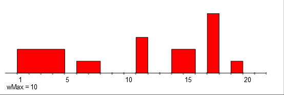
The following are two temporal quantities a and b represented in Python as a list of triples

a = [(1, 5, 2), (6, 8, 1), (11, 12, 3), (14, 16, 2), (17, 18, 5), (19, 20, 1)]
b = [(2, 3, 4), (4, 7, 3), (9, 10, 2), (13, 15, 5), (16, 21, 1)]

The temporal quantity a has on the interval [1,5) value 2, on the interval [6,8) value 1, on the interval [11,12) value 3, etc. Outside the specified intervals its value is undefined, ⌘.

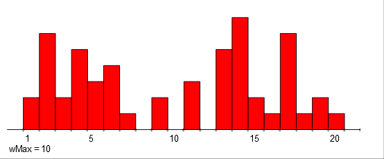
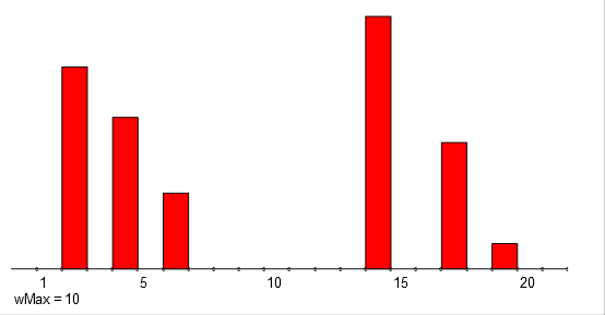
The temporal quantities can also be visualized as it is shown for a and b at the top half of the following figure:

Addition and multiplication of temporal quantities.

For the simplified version of temporal quantities we wrote procedures sum for the addition and prod for the multiplication of temporal quantities over the selected semiring. Because, by assumption, the triples in a description of a temporal quantity are ordered by their starting times, we can base both procedures on the ordered lists merging scheme. The basic semiring operations of addition and multiplication are provided by functions sAdd and sMul.

The following are the sum s and the product p of temporal quantities a and b.

s = [(1, 2, 2), (2, 3, 6), (3, 4, 2), (4, 5, 5), (5, 6, 3), 
     (6, 7, 4), (7, 8, 1), (9, 10, 2), (11, 12, 3), (13, 14, 5),
     (14, 15, 7), (15, 16, 2), (16, 17, 1), (17, 18, 6), 
     (18, 19, 1), (19, 20, 2), (20, 21, 1)]
p = [(2, 3, 8), (4, 5, 6), (6, 7, 3), (14, 15, 10), (17, 18, 5),
     (19, 20, 1)] 

They are visually displayed at the bottom half of the figure.

The function len(a) returns the length (number of items) of the list a. The function standard(a) joins, in the list a, adjacent time intervals with the same value into a single interval.

>>> TQ.combinatorial()
>>> a = [(1, 5, 2), (6, 8, 1), (11, 12, 3), (14, 16, 2), (17, 18, 5), (19, 20, 1)]
>>> b = [(2, 3, 4), (4, 7, 3), (9, 10, 2), (13, 15, 5), (16, 21, 1)]
>>> s = TQ.sum(a,b)
>>> s
[(1, 2, 2), (2, 3, 6), (3, 4, 2), (4, 5, 5), (5, 6, 3), (6, 7, 4),
 (7, 8, 1), (9, 10, 2), (11, 12, 3), (13, 14, 5), (14, 15, 7), (15, 16, 2),
 (16, 17, 1), (17, 18, 6), (18, 19, 1), (19, 20, 2), (20, 21, 1)]
>>> p = TQ.prod(a,b)
>>> p
[(2, 3, 8), (4, 5, 6), (6, 7, 3), (14, 15, 10), (17, 18, 5), (19, 20, 1)]
>>> len(p)
6
>>> c = [(1, 2, 2), (2, 3, 2), (4, 6, 2), (6, 8, 2)]
>>> TQ.standard(c)
[(1, 3, 2), (4, 8, 2)]
>>> 

Let l_a = len(a) and l_b = len(b). Then, assuming that the semiring operations take constant time each, the time complexity of both algorithms is O(l_a+l_b). The following example

shows that in extreme cases the sum can be almost 4 times longer than each of its arguments, and the product almost twice as long as the arguments. If T = [t_min, t_max] ⊆ ℕ the length of a list describing a temporal quantity can not exceed L = t_max - t_min.

In some applications over the combinatorial semiring we shall use the aggregated value of a temporal quantity a = ( (s_i, f_i, v_i) )_i∈1:k . It is defined as

∑a = ∑{i∈1:k : (f_i-s_i) ∙ v_i }

and is computed using the procedure total. For example ∑a = 23 and ∑b = 30. Note that ∑a + ∑b = ∑(a+b).

>>> a = [(1, 5, 2), (6, 8, 1), (11, 12, 3), (14, 16, 2), (17, 18, 5), (19, 20, 1)]
>>> TQ.total(a)
23
>>> 

We obtain a more adequate description of temporal networks by using vectors of temporal quantities (temporal vectors and temporal partitions) for describing properties of nodes and making also link weights into temporal quantities. In the current version of the library TQ we use a representation of a network N with its matrix A = [a_uv]

a_uv = w(u,v) if (u,v) ∈ L; and ⌘ otherwise

where w(u,v) is a temporal weight attached to a link (u,v).

The description of temporal partitions has the same form as the description of temporal quantities a = ( (s_i, f_i, v_i) )_i∈1:k. They differ only in the interpretation of values v_i ∈ ℕ. In case of partitions v_i = j means that the unit described with a belongs to a class j in the time interval [s_i,f_i). We shall use temporal partitions to describe connectivity components in Section~\ref{conn}.